Fusing Conv2d and BatchNorm2d
A common optimization technique in computer vision is fusing Conv2d and BatchNorm2d layers into a single Conv2d layer. This method is used by many optimization frameworks, such as TensorRT and ONNX Runtime. To understand how this is achieved, we’ll express these layers mathematically and demonstrate that applying batch normalization after a convolution is equivalent to a single convolution with adjusted parameters.
For a detailed introduction to batch normalization, I recommend Andrej Karpathy’s video.
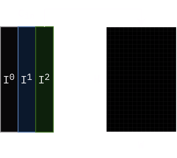
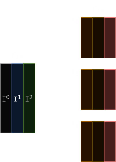
Let’s define our input \(I\) which is a 3-dimensional tensor \(C_{in}\) x \(H\) x \(W\) where \(C_{in}\) is the number of channels, \(H\) and \(W\) are height and width of the input respectively. Let’s say that \(I^{(k)}\) refers to k-th channel of \(I\). Each channel of \(I\) is a \(H\) x \(W\) tensor.
Convolutional layer consists of several filters. Each filter is a 3-dimensional tensor \(C_{in}\) x \(K\) x \(K\) where \(K\) is filter size and \(C_{in}\) is the number of input channels to the layer. We will denote \(i\)-th filter as \(F_i\) and refer to its \(k\)-th channel as \(F_i^k\).
Now, convolutional layer can be described as follows:
\[\begin{equation} C_{out}^i = \sum_{k=0}^{C_{in} - 1} I^{k} \circledast F^{k}_{i} + b^{i} \end{equation}\]Note that summation here operates on 2D matrices rather than scalars.
where \(C_{out}^i\) is the \(i\)-th channel of our output tensor, which is also a 3-dimensional tensor. \(I^{k} \circledast F^{k}_{i}\) denotes cross-correlation of input channel \(k\) with \(k\)-th channel of filter \(F_i\). \(b^{i}\) is bias of \(i\)-th filter.
Batch normalization is performed per-channel, so normalized output of channel \(C_{out}^i\) is:
\[y^{i} = \frac{C_{out}^i - E\left[ C_{out}^i \right]}{\sqrt{V \left[ C_{out}^i \right] + \epsilon }} \gamma^i + \beta^i\]where \(E[x]\) is running mean and \(V[x]\) is running variance in batch normalization layer. They are computed during training by BatchNorm2d layer using EMA. \(\epsilon\) is a small value added to avoid division by 0. \(\gamma^i\) and \(\beta^i\) are weight and bias of the batch normalization layer.
For simplicity, let’s define
\[\sigma^{-1}_i = \frac{1}{\sqrt{V \left[ C_{out}^i \right] + \epsilon }}\]Then, our batch normalization expression becomes:
\[y^{i} = \gamma^i \sigma^{-1}_i \left[ C_{out}^i - E[C_{out}^i] \right] + \beta^i\]Distributing \(\gamma^i \sigma^{-1}_i\) into the brackets we get the following expression:
\[y^{i} = \gamma^i \sigma^{-1}_i C_{out}^i - \gamma^i \sigma^{-1}_i E[C_{out}^i] + \beta^i\]Let’s take a closer look at the first term:
\[\gamma^i \sigma^{-1}_i C_{out}^i = \gamma^i \sigma^{-1}_i \left[ \sum_{k=0}^{C_{in} - 1} F_i^k \circledast I^k + b^i \right] = \sum_{k=0}^{C_{in} - 1} \gamma^i \sigma^{-1}_i \left(F_i^k \circledast I^k \right) + \gamma^i \sigma^{-1}_i b^i\]We are interested in the term \(\gamma^i \sigma^{-1}_i \left(F_i^k \circledast I^k \right)\).
\[\gamma^i \sigma^{-1}_i \left(F_i^k \circledast I^k \right) = \left(\gamma^i \sigma^{-1}_i F_i^k \right) \circledast I^k.\]We can make an observation about cross-correlation. Suppose we have two 2-dimensional matrices \(A\) of size \(H\) x \(W\) and \(B\) of size \(k\) x \(k\). Element \((i,j)\) of their cross-correlation is defined as:
\[\left( A \circledast B \right)_{i,j} = \sum_{m=0}^{k-1}\sum_{n=0}^{k-1} A_{i+m,j+n}B_{i,j}\]Let’s now multiply the cross-correlation by a scalar \(p\):
\[p \times \left( A \circledast B \right)_{i,j} = \sum_{m=0}^{k-1}\sum_{n=0}^{k-1} pA_{i+m,j+n}B_{i,j}\]which is the same as \(\left( \left( pA\right) \circledast B \right) _{i,j}\), therefore we can use this property:
\[p \times \left( A \circledast B \right)_{i,j} = \left( \left(pA\right) \circledast B \right)_{i,j}\]
Our final equation for batch normalization then becomes:
\[y^i = \sum_{k=0}^{C_{in} - 1} \left(\gamma^i \sigma^{-1}_i F_i^k \right)\circledast I^k + \gamma^i \sigma^{-1}_i b^i - \gamma^i \sigma^{-1}_i E[C_{out}^i] + \beta^i\]Let’s denote
\[\gamma^i \sigma^{-1}_i F_i^k = \hat{F}^k_i\]and
\[\gamma^i \sigma^{-1}_i b^i - \gamma^i \sigma^{-1}_i E[C_{out}^i] + \beta^i = B^i\]Then, equation can be expressed as:
\[y^i = \sum_{k=0}^{C_{in} - 1} \hat{F}^k_i \circledast I^k + B^i\]which is exactly the form that we started with. In the end, we rearranged the equation to show that batch normalization after a convolution can be expressed by a single convolution with weight \(\hat{F}^k_i = \gamma^i \sigma^{-1}_i F_i^k\) and bias \(B^i = \gamma^i \sigma^{-1}_i b^i - \gamma^i \sigma^{-1}_i E[C_{out}^i] + \beta^i\).
Let’s now put it to the test.
import torch as th
import torch.nn as nn
We will create a simple model with a Conv2d followed by a BatchNorm2d:
conv = nn.Conv2d(3, 64, 3)
norm = nn.BatchNorm2d(64).eval()

model = nn.Sequential(conv, norm)
For reference, we will generate a random input tensor and calculate our ground truth:
x = th.rand(1, 3, 64, 64)
y_gt = model(x)
Now let’s create a fused convolution by following the equations above:
conv_norm_fused = nn.Conv2d(3, 64, 3)

inv_sigma = 1 / th.sqrt(norm.running_var + norm.eps)
conv_norm_fused.weight.data = (norm.weight * inv_sigma).reshape(-1, 1, 1, 1) * conv.weight
conv_norm_fused.bias.data = norm.weight * inv_sigma * conv.bias - norm.weight * inv_sigma * norm.running_mean + norm.bias
y_fused = conv_norm_fused(x)
To test the output, let’s find the maximum absolute difference between y_fused and y_gt:
(y_fused - y_gt).abs().max()
tensor(4.1723e-07, grad_fn=<MaxBackward1>)
We still get a tiny error due to numerical stability reasons. However, it’s close enough to assume that they are equal.